POMS.6120 - Statistic for Predictive Analytics
Multiple Regression on Boston Dataset
A Step by Step Walkthrough
KEY QUESTIONS
Load the library(ISLR2) Boston Dataset
Describe Plot Findings (pairwise scatterplots, boxplots, and histograms)
Fit a multiple regression model to the training set (80/20 Split) to predict per capita crime rate using all the predictors
Fit a best subset selection to the training set to predict per capita crime rate (K-Fold added as well)
Fit LASSO to the training set to predict per capita crime rate
Apply smoothing spline to one or more predictors.
Fit a model to the training set to predict per capita crime rate using gam()
Use ANOVA to compare among various models
Which of the above models seem to perform well on this dataset? Justify your answers.
STEP 1
Load the Data
Load the library(ISLR2) Boston Dataset
DATA QUALITY: BOSTON DATASET
The Boston dataset from the ISLR2 library has been pre-scrubbed, cleansed, and verified to be free of missing values sum(colSums(is.na(df))) = 0 and duplicate records . The columns (variables) are all numeric data types. No additional data quality management was required.
We first load the library that contains the boston dataset library(ISLR2) and set df <- Boston along with df_name <- "Boston Dataset" which is a friendly title name for the subsequent charts.Next since some plots only like numeric and/or categorical columns, we create two new dataframes for the two different datatype that exist.Numeric Dataframe
df_columns\_numeric <- df[, sapply(df, is.numeric)]Categorical Dataframe
df_columns\_string <- df[, !sapply(df, is.numeric)]
| 506 |
|---|
| Rows of Data |
DATA DICTIONARY
| Column | Description | Value |
|---|---|---|
| crim | per capita crime rate by town. | 0.00632 |
| zn | proportion of residential land zoned for lots over 25,000 sq.ft. | 18 |
| indus | proportion of non-retail business acres per town. | 2.31 |
| chas | Charles River dummy variable (= 1 if tract bounds river; 0 otherwise). | 0 |
| nox | nitrogen oxides concentration (parts per 10 million). | 0.538 |
| rm | average number of rooms per dwelling. | 6.575 |
| age | proportion of owner-occupied units built prior to 1940. | 65.2 |
| dis | weighted mean of distances to five Boston employment centres. | 4.0900 |
| rad | index of accessibility to radial highways. | 1 |
| tax | full-value property-tax rate per $10,000. | 296 |
| ptratio | pupil-teacher ratio by town. | 15.3 |
| lstat | lower status of the population (percent). | 4.98 |
| medv | median value of owner-occupied homes in $1000s. | 24.0 |
STEP 2
Describe Plot Findings
Describe Plot Findings (pairwise scatterplots, boxplots, and histograms)
ANALYZE: PAIRWISE SCATTER PLOT
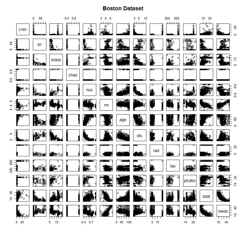
While pairwise scatter plots are great to get an overall sense of the distribution, since many columns have a low number of distinct values (whether qualitative or quantitative) and we can already see distinct correlations between lstat amd medv, among others. And at 78 unique pairs (since we exclude the pairs unto themselves), our job is to use the methods below to see beyond what the human eye can identify and discover potential non-visible patterns and correlations.
> ### pairwise_scatter_plots
> pairs(~ ., data = df, main = df_name)
ANALYZE: BOX PLOT
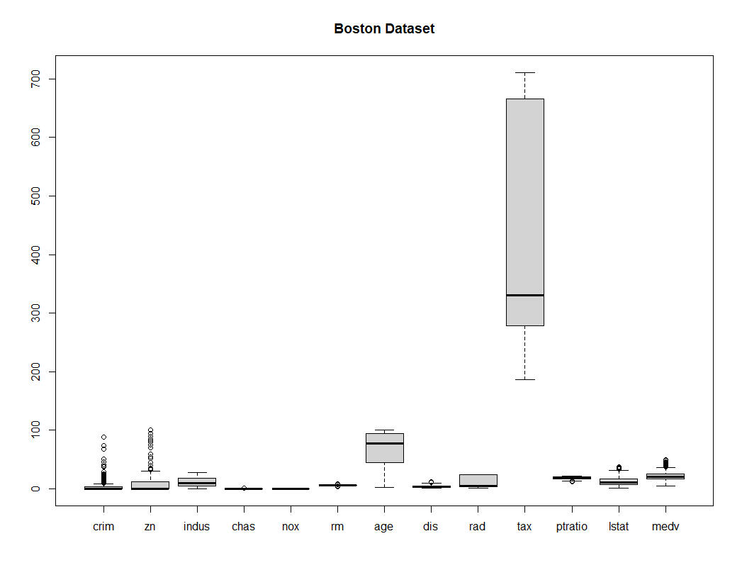
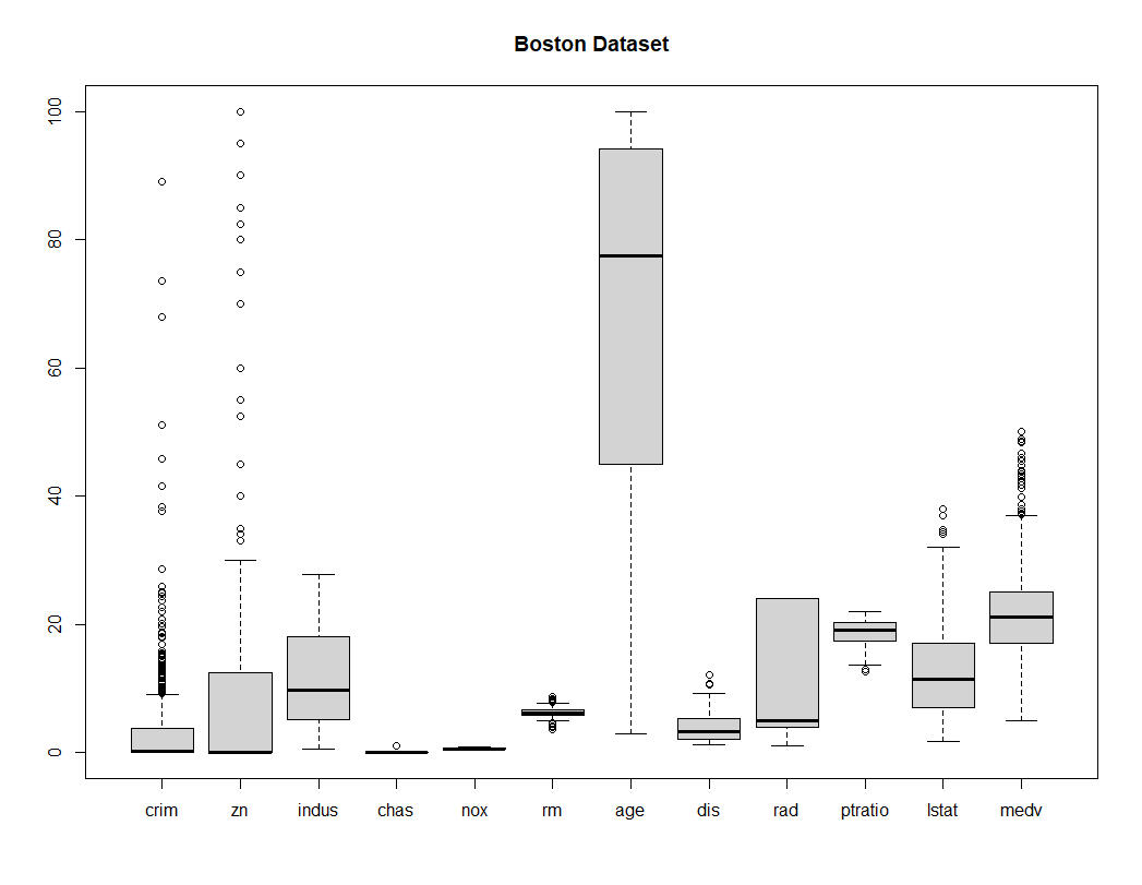
This type of plot is great at easily identifying if the data overalps one another or not.By plotting all of the columns using theboxplot(df, main = df_name) function, we can immediately see that tax is the only column that doesn't overlap.Removing Tax from he box plot, we now see clearly that age doesn't overlap with the rest of the columns.The rest appear in the range of 0 to 100.
Box 1: All Columns
Box 2: "Tax" Removed
ANALYZE: HISTOGRAM
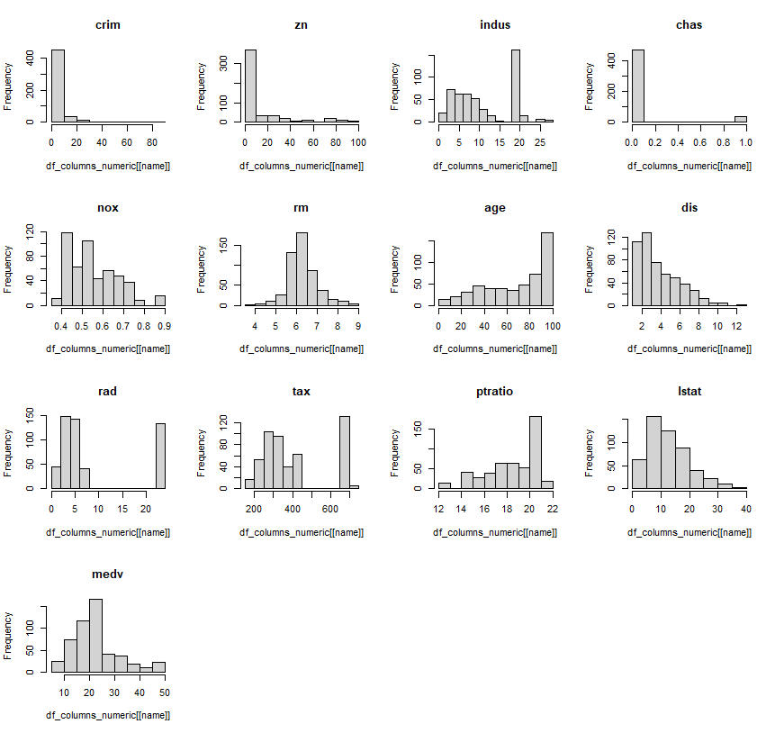
Crim which is the estimate, is heavily skewed with a right tail, with zn being the only other distribution that has similar patterns. Rad and tax have potential outliers at the right tail, and the rest of the bins and counts are unimodal and bimodal.
> ### histogram_plots
> par(mfrow = c(4, 4))
> for (name in names(df_columns_numeric)) {
+ hist(df_columns_numeric[[name]], main = name)
+ }
> par(mfrow = c(1, 1))
STEP 3A
Multiple Regression Model
Fit a multiple regression model to the training set (80/20 Split) to predict per capita crime rate using all the predictors
SPLIT DATA: TRAIN AND TEST
| 405 |
|---|
| Training Data |
| 101 |
|---|
| Test Data |
> set.seed(6)
>
> # 80/20 split for training/test
>
> n <- nrow(Boston)
>
> trainid<-sample(1:n, size=floor(0.8*n),replace=FALSE)
>
> train<-Boston[trainid,]
>
> test<-Boston[-train_id,]
TRAINING DATA: COEFFICIENT TABLEWe assign ŷ = the "crim" column in our Boston dataframe to be what we're estimating using all other columns as predictors β̂ₚXₚ with the intercept β̂₀ being ŷ when all other columns Xₚ = 0.In RStudio the code does the heavy lifting.lm.fit = lm(crim ~ ., data = train)Using the training dataframe only, we output as a table the multiple linear regression tablesummary(lm.fit)The (Intercept) is the Y value when all predictors Xp are 0.At a significance level of p-value < 0.001 only three columns account for any type of significant effect on the response variable.Therefore, we fail to reject the null hypothesis H₀: βⱼ = 0 for these columns from the Boston dataset.
| Columns | Estimate | Std. Error | t-value | p-value | Signif |
|---|---|---|---|---|---|
| (Intercept) | 17.719231 | 8.511276 | 2.082 | 0.038006 | * |
| zn | 0.050072 | 0.022690 | 2.207 | 0.027910 | * |
| indus | -0.067138 | 0.099724 | -0.673 | 0.501193 | |
| chas | -0.808211 | 1.433208 | -0.564 | 0.573134 | |
| nox | -14.051109 | 6.407189 | -2.193 | 0.028894 | * |
| rm | 0.687317 | 0.725448 | 0.947 | 0.344001 | |
| age | 0.005772 | 0.022075 | 0.261 | 0.793864 | |
| dis | -1.211296 | 0.348819 | -3.473 | 0.000573 | *** |
| rad | 0.646821 | 0.101973 | 6.343 | 6.23e-10 | *** |
| tax | -0.004695 | 0.006072 | -0.773 | 0.439838 | |
| ptratio | -0.354194 | 0.224718 | -1.576 | 0.115795 | |
| lstat | 0.138341 | 0.090033 | 1.537 | 0.125212 | |
| medv | -0.251744 | 0.072196 | -3.487 | 0.000544 | *** |
| Columns | p-value | Signif | |
|---|---|---|---|
| (Intercept) | 17.719231 | 0.038006 | * |
| zn | 0.050072 | 0.027910 | * |
| indus | -0.673 | 0.501193 | |
| chas | -0.564 | 0.573134 | |
| nox | -2.193 | 0.028894 | * |
| rm | 0.947 | 0.344001 | |
| age | 0.261 | 0.793864 | |
| dis | -3.473 | 0.000573 | *** |
| rad | 6.343 | 6.23e-10 | *** |
| tax | -0.773 | 0.439838 | |
| ptratio | -1.576 | 0.115795 | |
| lstat | 1.537 | 0.125212 | |
| medv | -3.487 | 0.000544 | *** |
TRAINING DATA: MODEL FIT TABLENext we examine the Model Fit Summary Table and other key statistical outputs from the RStudio code we entered in above.R2 = 0.43 is a moderately weak fit.43% of the variance in the response variable are explained by the predictors.Adjusted R2 is close to the actual R-Squared, so we know at least that the predictors with higher p-value are not penalizing predictors that are contributing to the variance.
| Metric | Value |
|---|---|
| R² | 0.4364 |
| Adjusted R² | 0.4191 |
| Residual Std. Error | 6.977 (df = 391) |
| F-statistic | 25.23 (12 and 391 DF) |
| F p-value | <2.2e-16 |
| Residual Min | -9.258 |
| Residual 1Q | -2.571 |
| Residual Median | -0.395 |
| Residual 3Q | 1.217 |
| Residual Max | 73.292 |
The F-statistic p-value of 2.2e-16 < 0.001 signifies that even though R2 is moderately weak, there's still value in the overall model describing the variance of the response variable "crim."And finally, the Residuals tell the potential story that the line of best fit model has outliers and a tail.The Residual MAX of 73.292 means that the model is not capturing high crime rate, and the distribution is right tailed since 3Q is 1.217and close to the median.A Residual Median of -0.395 and 1Q -2.571 confirms this.We now can conclude that further model fit analysis is required to see if we can account for the model not accurately capturing right tailed residual datapoints.
STEP 3B
Residual Analysis
Optional & TBD
STEP 4
Best Subset Selection
Fit a best subset selection to the training set to predict per capita crime rate
EXHAUSTIVE: BEST SUBSET SELECTIONWe let M0 denote the null model and set nvmax = 12 so that best subset selection considers models of every size k = 1...12.regfit.full <- regsubsetsWe call the regsubsets function using the library(leaps), assign the same train data.frame from above, and since there's only 212 possibilities, we are free to start with the
(
crim ~ ., train,
nvmax = 12,
method = "exhaustive"
)"exhaustive" method to truly find the best subset using all combinations of p.
| Model | zn | indus | chas | nox | rm | age | dis | rad | tax | ptratio | lstat | medv |
|---|---|---|---|---|---|---|---|---|---|---|---|---|
| 1 | . | . | . | . | . | . | . | [*] | . | . | . | . |
| 2 | . | . | . | . | . | . | . | [*] | . | . | [*] | . |
| 3 | . | . | . | . | . | . | . | [*] | . | . | [*] | [*] |
| 4 | [*] | . | . | . | . | . | [*] | [*] | . | . | . | [*] |
| 5 | [*] | [*] | . | . | . | . | [*] | [*] | . | . | . | [*] |
| 6 | [*] | . | . | [*] | . | . | [*] | [*] | . | [*] | . | [*] |
| 7 | [*] | . | . | [*] | . | . | [*] | [*] | . | [*] | [*] | [*] |
| 8 | [*] | [*] | . | [*] | . | . | [*] | [*] | . | [*] | [*] | [*] |
| 9 | [*] | [*] | . | [*] | [*] | . | [*] | [*] | . | [*] | [*] | [*] |
| 10 | [*] | [*] | . | [*] | [*] | . | [*] | [*] | [*] | [*] | [*] | [*] |
| 11 | [*] | [*] | [*] | [*] | [*] | . | [*] | [*] | [*] | [*] | [*] | [*] |
| 12 | [*] | [*] | [*] | [*] | [*] | [*] | [*] | [*] | [*] | [*] | [*] | [*] |
Next we switch to the "forward" subset selection method.
| Model | zn | indus | chas | nox | rm | age | dis | rad | tax | ptratio | lstat | medv |
|---|---|---|---|---|---|---|---|---|---|---|---|---|
| 1 | . | . | . | . | . | . | . | [*] | . | . | . | . |
| 2 | . | . | . | . | . | . | . | [*] | . | . | [*] | . |
| 3 | . | . | . | . | . | . | . | [*] | . | . | [*] | [*] |
| 4 | . | . | . | . | . | . | . | [*] | . | [*] | [*] | [*] |
| 5 | . | . | . | [*] | . | . | . | [*] | . | [*] | [*] | [*] |
| 6 | . | . | . | [*] | . | . | [*] | [*] | . | [*] | [*] | [*] |
| 7 | [*] | . | . | [*] | . | . | [*] | [*] | . | [*] | [*] | [*] |
| 8 | [*] | [*] | . | [*] | . | . | [*] | [*] | . | [*] | [*] | [*] |
| 9 | [*] | [*] | . | [*] | [*] | . | [*] | [*] | . | [*] | [*] | [*] |
| 10 | [*] | [*] | . | [*] | [*] | . | [*] | [*] | [*] | [*] | [*] | [*] |
| 11 | [*] | [*] | [*] | [*] | [*] | . | [*] | [*] | [*] | [*] | [*] | [*] |
| 12 | [*] | [*] | [*] | [*] | [*] | [*] | [*] | [*] | [*] | [*] | [*] | [*] |
Here we can see both method of subset selection start off the same.
rad
rad, lstat
rad, lstat, medv
But at selection 4 they start to diverge in predictors selected.
> coef(subsetexhausted, 4)
(Intercept) zn dis rad medv
5.95512764 0.06149382 -0.80938063 0.49954137 -0.20913186> coef(subsetforward, 4)
(Intercept) rad ptratio lstat medv
5.4649174 0.5585922 -0.3307542 0.1476865 -0.1297193> coef(subset_backward, 4)
(Intercept) zn dis rad medv
5.95512764 0.06149382 -0.80938063 0.49954137 -0.20913186
And running "backwards" subset selection It diverges at model 2 where backward picks medv instead of lstat!
| Model | zn | indus | chas | nox | rm | age | dis | rad | tax | ptratio | lstat | medv |
|---|---|---|---|---|---|---|---|---|---|---|---|---|
| 1 | . | . | . | . | . | . | . | [*] | . | . | . | . |
| 2 | . | . | . | . | . | . | . | [*] | . | . | . | [*] |
| 3 | . | . | . | . | . | . | [*] | [*] | . | . | . | [*] |
| 4 | [*] | . | . | . | . | . | [*] | [*] | . | . | . | [*] |
| 5 | [*] | . | . | [*] | . | . | [*] | [*] | . | . | . | [*] |
| 6 | [*] | . | . | [*] | . | . | [*] | [*] | . | [*] | . | [*] |
| 7 | [*] | . | . | [*] | . | . | [*] | [*] | . | [*] | [*] | [*] |
| 8 | [*] | [*] | . | [*] | . | . | [*] | [*] | . | [*] | [*] | [*] |
| 9 | [*] | [*] | . | [*] | [*] | . | [*] | [*] | . | [*] | [*] | [*] |
| 10 | [*] | [*] | . | [*] | [*] | . | [*] | [*] | [*] | [*] | [*] | [*] |
| 11 | [*] | [*] | [*] | [*] | [*] | . | [*] | [*] | [*] | [*] | [*] | [*] |
| 12 | [*] | [*] | [*] | [*] | [*] | [*] | [*] | [*] | [*] | [*] | [*] | [*] |
Since we CAN run the exhaustive subset selection, we know we have identified the best selection per model.Now we can identify the best model out of all exhaustive selections.
RSS and R2 will always have the model with all the predictors as either the highest R2 or lowest RSS because it is related to the training error.
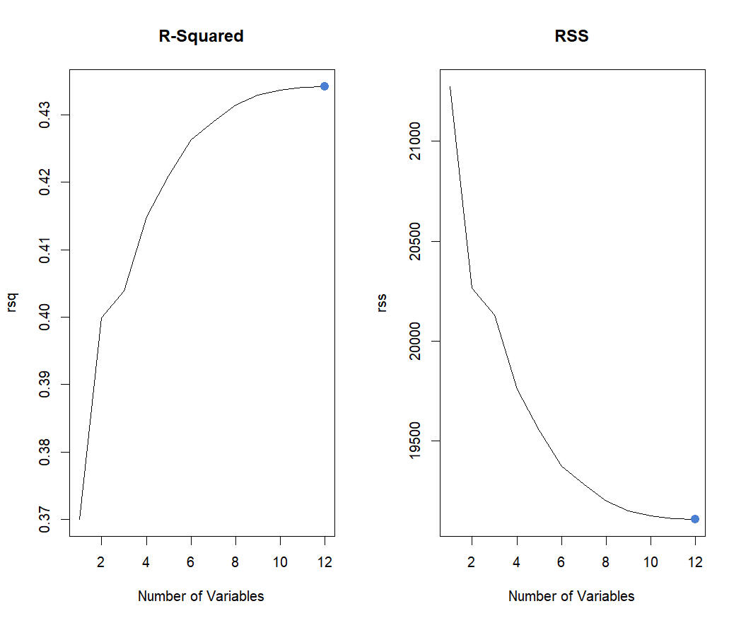
We care about test data. Therefore Cp, AIC (not shown since for linear models it's proportional to Cp), BIC, and Adjusted R2 are to be used.
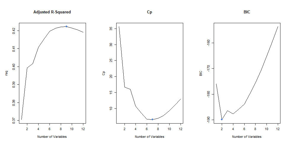
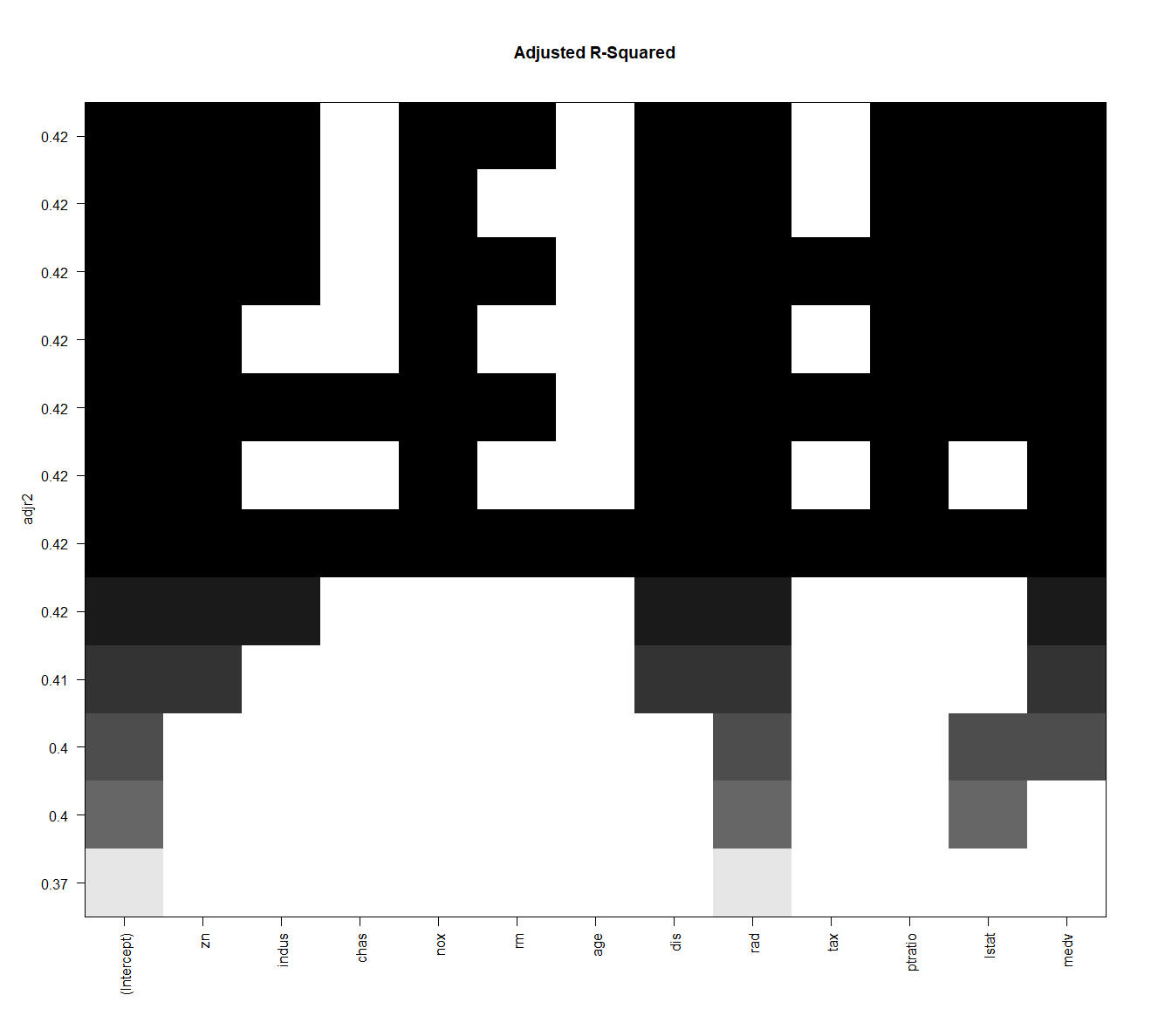
Adjusted R-Squared: 9
which.max(exhaustive_subset_summary$adjr2)
While R-Squared says that the model with 9 variables produces the highest adjusted value, we can see the plateau around 6 variables which matches Cp. Reinforcing that there's a clear cutoff at 6 variables no matter the model methodology.
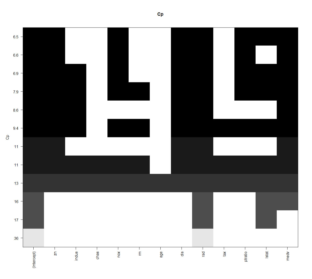
Cp: 7
which.min(exhaustive_subset_summary$cp)
The number of variables for Cp confirms just as R-Squared did that the number of variables is 6/7 and below.
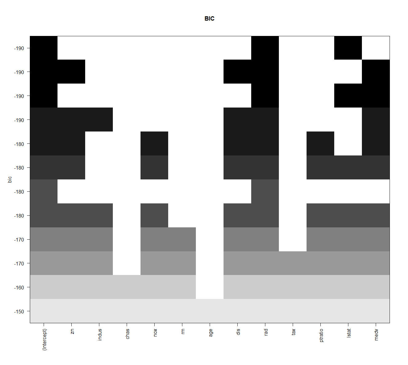
BIC: 2
which.min(subset_selected_summary$bic))
The Bayesian Information Criterion (BIC) says that we use 2 variables.
MODEL SELECTION: K-FoldWe begin by creating a function so that we do not have to keep on writing out the prediction code for regsubsets since it doesn't come included.predict.regsubsets <- function(object, newdata, id, ...)Next we implement the K-Fold code below, with the same Step by Step walkthrough afterwards.
{
form <- as.formula(object$call[[2]])
mat <- model.matrix(form, newdata)
coefi <- coef(object, id = id)
xvars <- names(coefi)
mat[, xvars] %*% coefi
}k <- 10Step 1: Assing k = 10 and n = number of row from data.frameStep 2: Seed(1) againStep 3: rep(creates a vector of length n, and sequentially assigns it 1 to k or 1 to 10 is all...) if you just passed rep(1:10) it's a vector of one sequential 1 to 10. Wrapping it in sample() randomized the entire index of length n.Step 4: cv.errors gets a matrix filled with NA’s that’s k=10 rows and 12 columnsStep 5: loops for j in 1:10 or 10 times…Step 5a: within the loop assign object best.fit <- the regsubsets() call passing crim as the estimate with the data being all from the data.frame that don’t come from the sample group j. once again nvmax = 12 combinatorial incremental subsets.Step 6: Within the prior loop of j in 1:k or 10, there’s the loop of 1 to 12 as i++. This is where the predict() of fold == j, where once again it grabs the coefficients from best.fit object for id position i.Step 7: Next once again cv.errors this time is fed the jth,ith column row position of the mean of the dataframe crim from the current fold j in the loop, and subtracting it from the prediction and squaring to get the Mean Squared Error for the jth fold of the ith variable subset.Step 8: Takes the mean for each of the 12 columns with k rows from cv.errors which was assigned the completed loop j in 1:k with the second loop of I in 1:12
n <- nrow(df)
set.seed(6)
folds <- sample(rep(1:k, length = n))
cv.errors <- matrix(NA, k, 12,
dimnames = list(NULL, paste(1:12)))
for (j in 1:k) {
best.fit <- regsubsets(crim ~ .,
data = df[folds != j, ],
nvmax = 12)
for (i in 1:12) {
pred <- predict(best.fit, df[folds == j, ], id = i)
cv.errors[j, i] <-
mean((df$crim[folds == j] - pred)^2)
}
}
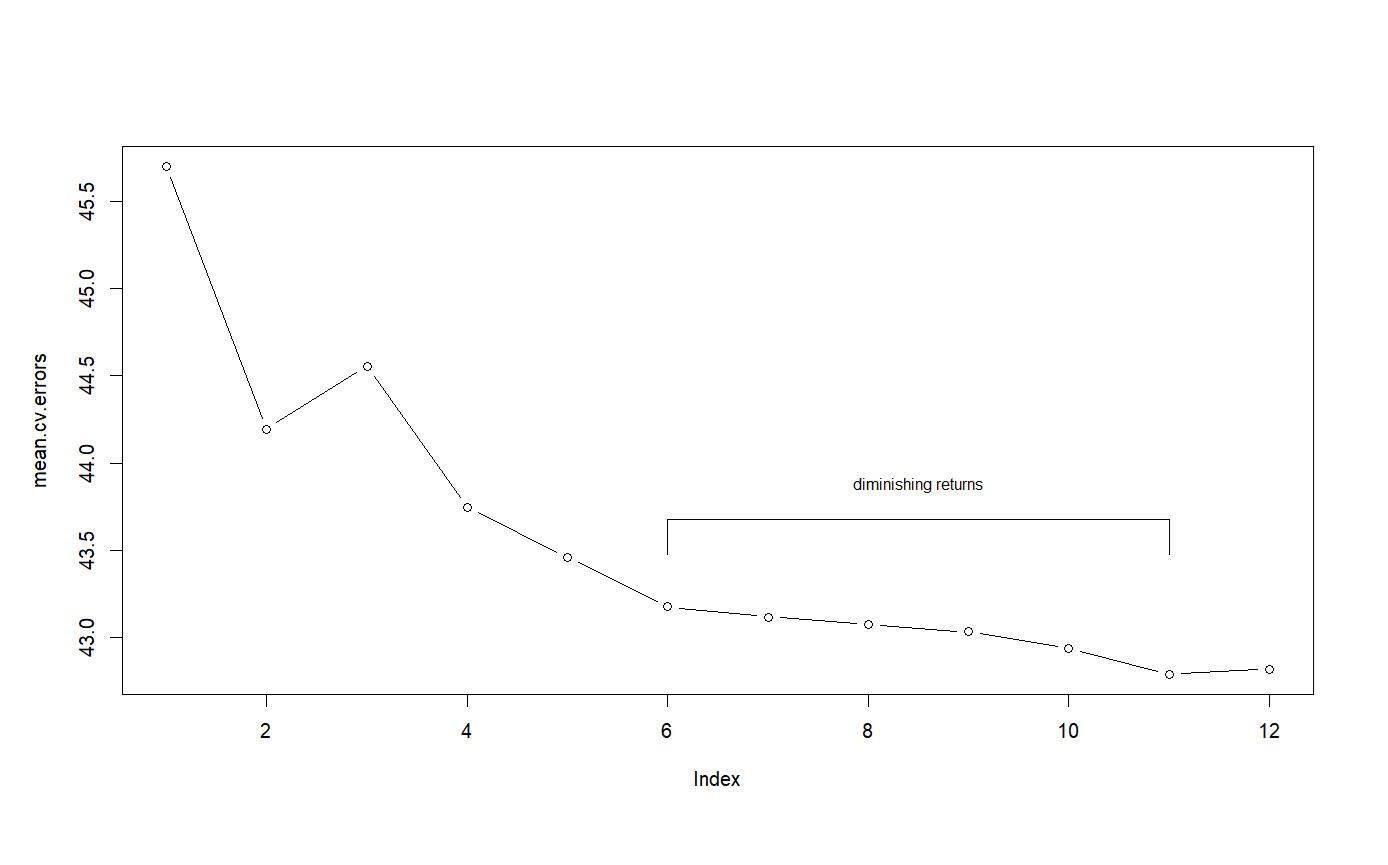
Step 9: Creates a plot of all the mean.cv.errors, so 12 datapoints of the average MSE from the jth fold of 12 combinatorial incremental subsets.We can see diminishing returns relative to lower MSE values on the y-axis past the 6th fold.
MODEL SELECTION: EXHAUSTIVE SUBSET SELECTIONWe begin by created a matrix table populated with the [test] data.frame.test.matrix <- model.matrix(crim ~ ., data = test)val.errors <- rep(NA, 12)for (i in 1:12)Step 1: val.errors is a vector of length 12 filled with NA'sStep 2: for i in 1:12loops 12 times doing i++Step 3: coefi <- coef() grabs the coefficients from subset_exhausted object for id position i start of the loop is 1Step 4: pred <- test.matrix[, names(coefi)] %% coefiWHERE test.matrix <- model.matrix(crim~ ., data = test)AND the pred object applying test.mat[, names(coefi)], the matrix we created of the intercept and all the variables... %% is multiplying each matrix columns actual value with the coefficient column of the same name using names(coefi) as the column "join."Step 5: Fill in for index i in val.errors <- rep(NA, 12) the average of the actual crim data from the test data.frame and subtract it from the prediction but square it so that positive and negative errors don't cancel each other out... And that's the estimated test errors (Mean Squared Errors) in a nutshell.Step 6: Is simply loop and do this for a total of 12 times.Step 7: is after the loop you have 12 Mean Squared Errors and val.errors below outputs all the MSE’s
{
coefi <- coef(subset_exhausted, id = i)
pred <- test.matrix[, names(coefi)] %*% coefi
val.errors[i] <- mean((test$crim - pred)^2)
}
> val.errors
[1] 15.17924 14.39851 14.29083 14.57155 15.06759 15.54896 15.42760 15.54248 15.63334 15.73215 15.67126 15.75243
MODEL WITH MINIMUM MSE: 3
which.min(val.errors)
> coef(subset_exhausted, 3)
(Intercept) rad lstat medv
-1.43918852 0.52798839 0.16546360 -0.09023959
We find that the best model is the one that contains three variables.This is well within the range of 2 to 6 using the best subset selection methodology and examining the R-Squared, Cp, and BIC recommended selection, along wiht K-Fold validating that a ceiling exists at 6.
EXPLORE MORE IDEAS
Copyright (C) ReqSquared. All Rights Reserved.
